What is Standard Deviation? Simple Explanation with Examples
Understand standard deviation with clear explanations, step-by-step calculations, and real-world examples. Learn the difference between population and sample standard deviation.
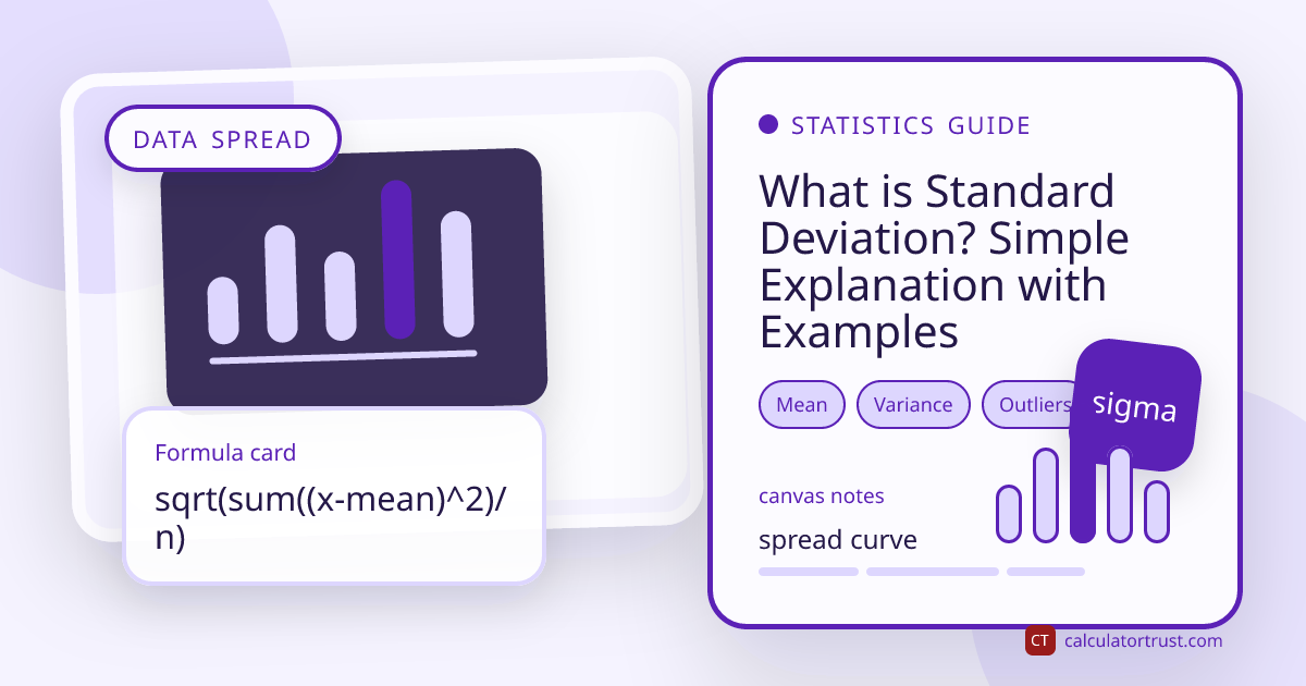
Standard deviation is one of the most important concepts in statistics, yet many people find it intimidating. At its heart, standard deviation answers a simple question: how spread out are the numbers in a data set? Whether you are analyzing test scores, investment returns, scientific measurements, or sports statistics, standard deviation gives you a single number that summarizes the variability of your data. In this guide, we will break down the concept, walk through the calculation step by step, explain the critical difference between population and sample standard deviation, and show you how it applies in the real world.
What Does Standard Deviation Measure?
Imagine two classes that both have an average test score of 75%. In Class A, every student scored between 70% and 80%. In Class B, scores ranged from 40% to 100%. Both classes have the same mean, but they are clearly very different. Standard deviation captures this difference — it measures how much individual values typically differ from the average.
A small standard deviation means the data points are clustered tightly around the mean, indicating consistency. A large standard deviation means the data points are spread widely, indicating diversity or variability. In our example, Class A would have a small standard deviation (scores are consistent) while Class B would have a large one (scores are all over the place).
Formally, standard deviation is defined as the square root of the average squared distance from the mean. That sounds complex, but each step has a clear purpose, as we will see when we walk through the calculation.
Think in typical distance
The easiest mental model is distance from the average. A larger standard deviation means a typical value sits farther from the mean.
Formula Snapshot
The core equation and the variables that control the answer.
The Standard Deviation Formula
There are two versions of the standard deviation formula depending on whether you are working with an entire population or a sample:
Population standard deviation (sigma): sigma = sqrt(sum((xi - mu)^2) / N)
Sample standard deviation (s): s = sqrt(sum((xi - x-bar)^2) / (n - 1))
Where:
Input Checklist
The values to collect before trusting the calculation.
- xi = each individual data point
- mu (or x-bar) = the mean of the data set
- N = the total number of data points (population)
- n = the number of data points in the sample
- sum = the sum across all data points
- sqrt = the square root
The only difference between the two formulas is the denominator: N for population, n-1 for sample. This distinction matters, and we will explain why in a later section.
Step-by-Step Calculation Example
Let us calculate the standard deviation of a small data set: the test scores 72, 85, 90, 68, and 95. We will use the sample standard deviation formula since this is likely a sample of students from a larger class.
Step 1: Find the mean.
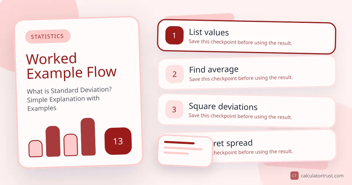
Worked Example Flow
A step-by-step flow for checking the math against real numbers.
Mean = (72 + 85 + 90 + 68 + 95) / 5 = 410 / 5 = 82
Step 2: Find each deviation from the mean.
- 72 - 82 = -10
- 85 - 82 = 3
- 90 - 82 = 8
- 68 - 82 = -14
- 95 - 82 = 13
Step 3: Square each deviation.
- (-10)^2 = 100
- (3)^2 = 9
- (8)^2 = 64
- (-14)^2 = 196
- (13)^2 = 169
Step 4: Find the sum of squared deviations.
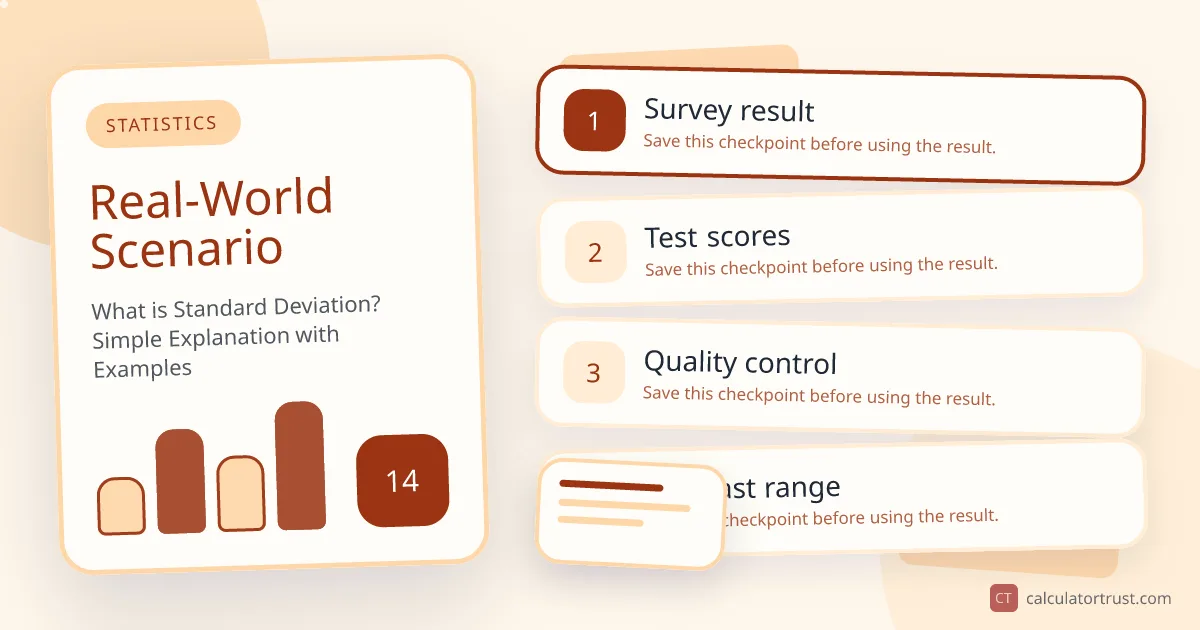
Real-World Scenario
How the calculation changes when real-life assumptions are included.
100 + 9 + 64 + 196 + 169 = 538
Step 5: Divide by n - 1 (this gives the variance).
Variance = 538 / (5 - 1) = 538 / 4 = 134.5
Step 6: Take the square root (this gives the standard deviation).
Standard deviation = sqrt(134.5) = 11.6
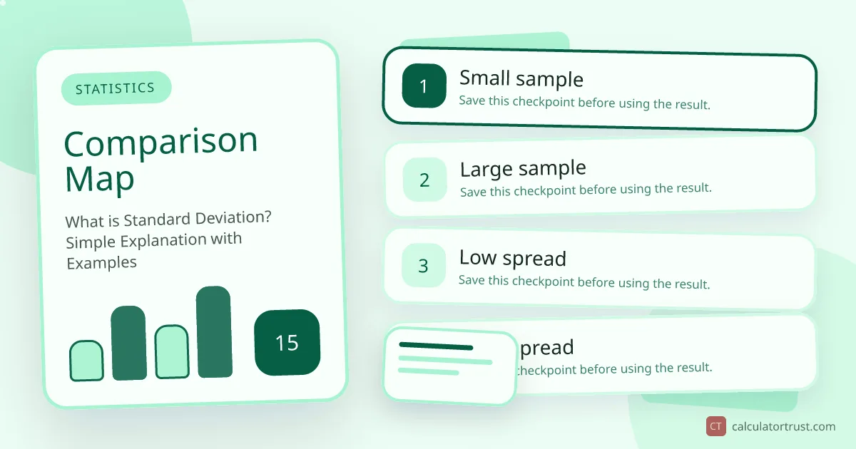
Comparison Map
A visual way to compare options, ranges, or outcomes.
The sample standard deviation is approximately 11.6 points, meaning scores typically deviate from the mean of 82 by about 11-12 points. You can verify this using our standard deviation calculator, which performs all six steps instantly for any data set.
Population vs. Sample Standard Deviation
The choice between population and sample standard deviation depends on your data:
- Population standard deviation (divide by N) is used when your data includes every member of the group you care about. For example, if you have the test scores of every student in a specific class and you only care about that class, use the population formula.
- Sample standard deviation (divide by n - 1) is used when your data is a subset of a larger group and you want to estimate the variability of the larger group. This is the more common scenario in statistics.
Why divide by n - 1 instead of n for samples? This is called Bessel's correction. A sample tends to underestimate the true population variability because sample data points are, on average, closer to the sample mean than to the true population mean. Dividing by n - 1 instead of n inflates the result slightly to correct for this bias, producing a more accurate estimate of the population standard deviation.
The difference between the two formulas is most significant for small samples. For a sample of 5, the difference is about 12%. For a sample of 30, it is about 1.7%. For a sample of 100, it is less than 0.5%. As your sample size grows, the two formulas converge.
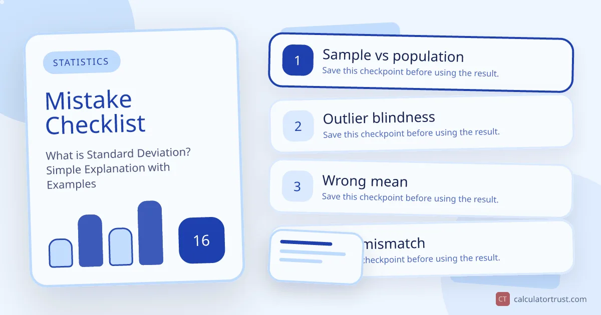
Mistake Checklist
Common errors that can make a correct formula produce a misleading result.
Understanding Variance
Variance and standard deviation are closely related — standard deviation is simply the square root of variance. Variance represents the average squared deviation from the mean. Squaring the deviations serves two purposes: it ensures that positive and negative deviations do not cancel each other out, and it gives extra weight to larger deviations (outliers).
While variance is mathematically convenient (it has useful properties in statistical analysis), its units are squared, which makes it harder to interpret. If test scores are measured in points, variance is in "points squared" — not very intuitive. Standard deviation brings the measurement back to the original units, making it directly interpretable.
In practice, standard deviation is used much more often than variance for reporting and interpretation. Variance is used more often in theoretical statistics and mathematical derivations.
The 68-95-99.7 Rule (Empirical Rule)
For data that follows a normal distribution (the familiar bell curve), standard deviation has a powerful interpretive property known as the empirical rule:
Quality Check
Simple checks for spotting a result that looks too high, low, or incomplete.
- Approximately 68% of values fall within 1 standard deviation of the mean
- Approximately 95% of values fall within 2 standard deviations of the mean
- Approximately 99.7% of values fall within 3 standard deviations of the mean
For our test score example with a mean of 82 and standard deviation of 11.6: about 68% of scores would fall between 70.4 and 93.6, about 95% would fall between 58.8 and 105.2, and virtually all scores would fall between 47.2 and 116.8.
This rule is incredibly useful for identifying outliers. Any value more than 2 standard deviations from the mean is unusual (only 5% of values fall there), and any value more than 3 standard deviations away is very rare (only 0.3% of values). This is the basis for many quality control systems and statistical tests.
Real-World Applications of Standard Deviation
Standard deviation appears across virtually every field that works with data:
Quick Reference
A compact checklist for using the guide and calculator together.
- Finance and investing: Standard deviation of returns is the primary measure of investment risk. A stock with an average annual return of 10% and a standard deviation of 20% is much riskier than one with the same average return and a standard deviation of 8%. Portfolio theory uses standard deviation to optimize the balance between risk and return.
- Manufacturing and quality control: Six Sigma methodology aims to keep product measurements within six standard deviations of the target value, resulting in a defect rate of only 3.4 per million items. Standard deviation directly determines whether a product passes or fails quality inspection.
- Education: Standard deviation helps teachers understand score distributions. A low standard deviation on a test might indicate that the material was well-taught and well-understood, while a high standard deviation might suggest that some students excelled while others struggled, pointing to a need for differentiated instruction.
- Weather and climate: Meteorologists use standard deviation to describe how unusual a temperature is. If the average July high in a city is 88°F with a standard deviation of 5°F, then a 100°F day is 2.4 standard deviations above the mean — a statistically unusual event.
- Healthcare: Lab results are often reported with reference ranges based on standard deviations from population means. A blood test result that falls more than 2 standard deviations from the normal mean may warrant further investigation.
Common Mistakes to Avoid
When working with standard deviation, watch out for these common errors:
- Using the wrong formula. Always determine whether you need population or sample standard deviation before calculating. Using the population formula on a sample will underestimate the true variability.
- Forgetting to square the deviations. Simply averaging the deviations from the mean gives zero because positive and negative deviations cancel out. Squaring is essential to capture the magnitude of spread.
- Comparing standard deviations of different scales. A standard deviation of 5 on a 0-10 scale indicates huge variability, while a standard deviation of 5 on a 0-1000 scale indicates almost no variability. Use the coefficient of variation (standard deviation divided by the mean) to compare variability between data sets of different scales.
- Assuming normality. The 68-95-99.7 rule only applies to normal distributions. For skewed or multimodal data, standard deviation still measures spread, but the empirical rule percentages do not hold.
Standard deviation is a foundational statistical concept that becomes intuitive with practice. Once you understand what it measures and how to calculate it, you will find yourself recognizing its applications everywhere — from reading financial reports to understanding medical test results. For quick calculations, our standard deviation calculator handles data sets of any size and shows both population and sample results.